
Maximize Signal Range and Wireless Monitoring Capability
 Wireless signal attenuation is the reduction of energy or a radio frequency (RF) transmission, such as when sending data via WiFi, Zigbee, or some communication protocol for applications such as automated temperature monitoring. Attenuation is represented in decibels (dB), which is ten times the logarithm of the signal power at a particular input or source location in watts divided by the output or receiving end of a specified medium. For example, an office wall (the specific medium) that changes the strength of an RF signal from a power level of 10 milliwatts (the input) to 5 milliwatts (the output) represents 3 dB of attenuation. Consequently, positive attenuation causes signals to become weaker when traveling through the medium.
When the attenuation is high, signal power decreases to relatively low values, and the receiving device can encounter errors when trying to decode the radio signal. This problem gets worse when there is significant RF interference from other equipment in the environment. For example, IEEE 802.11 or WiFi, Zigbee, and other devices often operate on the same 2.5 GHz industrial, scientific, and medical (ISM) band that is also shared with microwave ovens. The occurrence of bit errors may prevent the receiving station from properly decoding wireless packets and sending a receipt acknowledgment to the source station. After a short period of time, the sending station will retransmit the frame; to the user, this will appear as slow communications. In the worst case, signal power loss due to attenuation becomes so low that the system loses connectivity and all transmission stops.

A common signal strength indicator is the Link Quality Indication (LQI) measurement based on the bit error rate [BER] of the current packet being received. The BER is expressed as a percentage calculated from the number of corrupt bits over the total number of bits in an individual wireless data packet. In a mesh network like Zigbee, it is calculated based on the previous hop of the inbound route, so that it provides information specific to the link-layer connection to the neighboring device relaying the current packet to the local device.
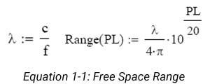
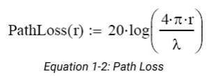
Any medium including air, water, wood, drywall, or concrete between the transmitter and receiver will cause attenuation of the signal strength and a reduction in the useable range between the endpoints. As the distance increases, attenuation also increases. Attenuation in outdoor applications is based on straightforward and basic free space calculations, but in contrast, indoor applications can be very complex to calculate. In both cases, loss formulas can be used (see Equation 1 and Equation 2). The main reason for the indoor difficulty is that signal may have to pass through a variety of materials that offer varying effects on attenuation (see Table 1-2 Obstacle attenuation) and that signals may bounce off different obstacles making the exact path difficult to determine.
Free Space Loss Formulas
Typical Path Losses To Be Added dB:
| Human body | 3 |
| Cubicles | 3 to 5 |
| Window, Brick Wall | 2 |
| Brick Wall next to a Metal Door | 3 |
| Glass Window (non-tinted) | 2 |
| Clear Glass Window | 2 |
| Office window | 3 |
| Plasterboard wall | 3 |
| Marble | 5 |
| Glass wall with metal frame | 6 |
| Metal Frame Glass Wall Into Building | 6 |
| Metal Frame Clear Glass Wall | 6 |
| Metal Screened Clear Glass Window | 6 |
| Wired-Glass Window | 8 |
| Cinder block wall | 4 |
| Dry Wall | 4 |
| Cinder Block Wall | 4 |
| Sheetrock/Wood Frame Wall | 5 |
| Sheetrock/Metal Framed Wall | 6 |
| Office Wall | 6 |
| Brick Wall | 2 to 8 |
| Concrete Wall | 10 to 15 |
| Wooden Door | 3 |
| Metal door | 6 |
| Metal Door in Office Wall | 6 |
| Metal door in brick wall | 12 to 13 |
| Table 1-2 Obstacle Signal Attenuation |

Because of the complexity of determining a result, it’s often best to perform an RF site survey to fully understand the behavior of radio waves within a facility before installing wireless devices. The ultimate goal of the survey is to supply enough information to determine the number and placement of wireless transmitters, receivers/network gateways, and potential repeaters to provide adequate coverage throughout the facility. An RF site survey also detects the presence of interference coming from other sources that could degrade the performance of the system.
The need and complexity of an RF site survey will vary depending on the facility, e.g. a small three-room office may not require a site survey—the site will probably get by with a single wireless network gateway located anywhere within the office and still maintain adequate coverage. A larger facility, such as a laboratory, hospital, or warehouse may require an extensive RF site survey to map coverage over a spread-out area or over multiple floors. Without a survey, the system may end up with inadequate coverage and suffer from low performance in some areas. When conducting an RF site survey, consider these general steps:
1. Obtain a facility diagram. Locate a set of building blueprints, if possible. If none are available, prepare a floor plan drawing that depicts the location of wood or concrete walls, stairways, etc.
2. Visually inspect the facility. Be sure to walk through the facility before performing any tests to verify the accuracy of the facility diagram. This is a good time to note any potential barriers that may affect the propagation of RF signals, e.g. a visual inspection will discover obstacles such as metal racks, cabinets, and partitions-items that blueprints don’t show.
3. Identify user areas. On the facility diagram, mark the areas where fixed and mobile pods are to be placed. In addition to illustrating where mobile pods may be moved around, also indicate where they will not be placed. The system may require fewer wireless network gateway points if roaming areas can be limited.
4. Determine preliminary access point locations. By considering the location of pods and range estimations between pods and gateways, estimate the locations of gateways to provide adequate coverage throughout the area (preliminary locations). Consider mounting locations, which could be vertical posts or metal posts above ceiling tiles. Be sure to recognize suitable locations for installing the access point, antenna, data cable, and power line. Also, think about different antenna types when deciding where to position access points. An access point mounted near an outside wall, for example, could be a good location if a patch antenna with a relatively high gain is oriented within the facility.
5. Verify access point locations. This is when the real testing begins: it’s a two-person job. Install a wireless network gateway at each location and monitor the signal strength indicator readings by walking with a pod for varying distances away from the access point. Take note of data rates and signal readings at different points as the pod is moved to the outer bounds of the gateway’s coverage. In a multi-floor facility, perform tests on the floor above and below the access point. Keep in mind that a poor signal quality reading likely indicates that RF interference is affecting the system. Based on the results of the testing, you might need to reconsider the location of some access points and retest the affected areas.
6. Document findings. Once you’re satisfied that the planned location of access points will provide adequate coverage, identify the recommended mounting locations on the facility diagram. The installers will need this information.
NOTE: Underground tunnels act as wave guides giving far greater ranges than aboveground. Metal ceilings have been found to behave similarly.
RF interference from other equipment can plague wireless system deployments. The perils of interfering signals from external RF sources are often the culprit. As a result, it’s important that you’re fully aware of any other equipment in the area that may operate on the same frequency band as the wireless system you are trying to deploy.
Signal Attenuation
RF signal fading is caused by several factors including Multipath Reception, Line of Sight Interference, Fresnel Zone Interference, RF Interference, and weather conditions.
Multipath Reception – The transmitted signal arrives at the receiver from different directions, with different path lengths, attenuation, and delays. An RF reflective surface, like a cement surface or roof surface, can yield multiple paths between antennas. The higher the antenna mount position from such surfaces, the lower the multiple path losses. The radio equipment in the 802.11.4 specification utilizes modulation schemes and reception methods such that multiple path problems are minimized.
Line of Sight Interference – A clear, straight line of sight between system antennas is absolutely required for a proper RF link reaching long distances outdoors. A clear line of sight exists if an unobstructed view of one antenna from the other antenna exists. A radio wave clear line of sight exists if a defined area around the optical line of sight is also clear of obstacles. In setting up wireless networks in buildings, propagation of the RF signal through walls and other items is a fact of life. If you recall the signal attenuation discussion earlier, we can evaluate the related losses. The preceding Table 1-2 presents loss values for typical items through which we want our networks to transmit and receive.
Fresnel Zone Interference – The Fresnel (FRAY-nel) Zone is a circular area perpendicular to and centered on the line of sight. If there are interfering objects within this zone, the portion of the radio signal which spreads out off-axis can bounce off these objects and arrive at the receiving location out of phase causing destructive interference. In radio wave theory, if 80% of the first Fresnel Zone is clear of obstacles, the wave propagation loss is equivalent to that of free space.
RF Interference – This was discussed earlier.
Weather Conditions – At 2.4GHz, most rain showers can be penetrated with ease.
System Operating Margin (SOM)
SOM (System Operating Margin), also known as fade margin, is the difference of the receiver signal level in dBm minus the receiver sensitivity in dBm. It is a measure of the safety margin in a radio link. A higher SOM means a more reliable over-the-air connection. It is usually recommended to include a minimum of 10dB to 20dB SOM.
Shadowing
Shadowing is the effect where the received signal power fluctuates due to objects moving within the propagation path between transmitter and receiver, for example, someone walking between the transmitter and receiver. These fluctuations are experienced on local-mean powers, that is, short-term averages can be used to remove fluctuations due to shadowing.
To put this in contrast, in most papers on mobile propagation, only ‘small-area shadowing’ is considered: log-normal fluctuations of the local-mean power are measured when the antenna moves over a distance of tens or hundreds of meters. Marsan et al. reported a median of 3.7dB for small-area shadowing. Preller and Koch measured local-mean powers at 10m intervals and studied shadowing over 500m intervals. The maximum standard deviation experienced was about 7dB, but 50% of all experiments showed shadowing of less than 4dB.
Link Budget
A link budget is the accounting of all of the gains and losses from the transmitter through the medium (free space, walls, etc.) to the receiver in the system. It takes into account the attenuation of the transmitted signal due to propagation, as well as the loss or gain due to the antenna. A simple link budget equation looks like this:
Received Power (dB) = Transmitted Power (dBm) + Gains (dB) – Losses (dB)
Equation 1-3 Link budget
Equation 1-3 Link budget
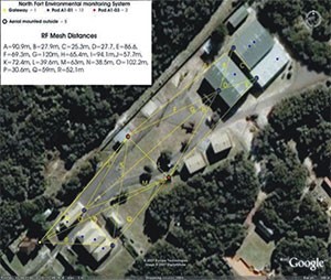
The example below shows the proposed layout for a wireless monitoring system for a museum installation with distances, pod type, and external antenna placement. The final system had an underground component and required 3 antennas above ground, taking into account roof skylights in three of the buildings, allowing RF signals to enter and exit.
The following table shows the link budget and margin calculations for the system. Note that distance G of 120m has a link budget that is reasonable but is calculated in the second half of the table to be outside the standard pod range; E and O are marginal.
Tx = transmitter
Rx = receiver
| Link | Distance (m) | Tx Pwr | Rx Sensitivity | Tx AntG | Tx Coax | Tx AntG | Rx Coax | Fading Margin | Loss | Link Budget |
| A | 90.9 | -1 | -94 | 9 | 0 | 9 | 0 | 18 | 5 | 88 |
| B | 27.9 | -1 | -94 | 9 | 0 | 9 | 0 | 18 | 12 | 81 |
| C | 25.3 | -1 | -94 | 9 | 0 | 9 | 0 | 18 | 11 | 82 |
| D | 27.7 | -1 | -94 | 9 | 0 | 9 | 0 | 18 | 11 | 82 |
| E | 86.6 | -1 | -94 | 9 | 3 | 9 | 0 | 18 | 5 | 85 |
| F | 69.3 | -1 | -94 | 9 | 0 | 9 | 0 | 18 | 6 | 87 |
| G | 120 | -1 | -94 | 9 | 0 | 9 | 0 | 18 | 11 | 82 |
| H | 65.4 | -1 | -94 | 9 | 3 | 9 | 0 | 18 | 5 | 85 |
| I | 94.1 | -1 | -94 | 9 | 0 | 9 | 0 | 18 | 5 | 88 |
| J | 57.7 | -1 | -94 | 9 | 0 | 9 | 0 | 18 | 5 | 88 |
| K | 72.4 | -1 | -94 | 9 | 3 | 9 | 0 | 18 | 5 | 85 |
| L | 39.6 | -1 | -94 | 9 | 3 | 9 | 0 | 18 | 0 | 90 |
| M | 63 | -1 | -94 | 9 | 3 | 9 | 0 | 18 | 5 | 85 |
| N | 38.5 | -1 | -94 | 9 | 0 | 9 | 0 | 18 | 10 | 83 |
| O | 102.2 | -1 | -94 | 9 | 3 | 9 | 0 | 18 | 5 | 85 |
| P | 30.6 | -1 | -94 | 9 | 0 | 9 | 0 | 18 | 10 | 83 |
| Q | 59 | -1 | -94 | 9 | 3 | 9 | 0 | 18 | 5 | 85 |
| R | 52.1 | -1 | -94 | 9 | 0 | 9 | 0 | 18 | 10 | 83 |
| Link | Range (m) | Margin (m) | Margin (db) | Shadowing | Link Budget | Range (m) | Margin (m) | Margin (db) |
| A | 241.6 | 150.7 | 8.5 | 3.7 | 84.3 | 157.8 | 66.9 | 4.8 |
| B | 107.9 | 80.0 | 11.8 | 3.7 | 77.3 | 70.5 | 42.6 | 8.1 |
| C | 121.1 | 95.8 | 13.6 | 3.7 | 78.3 | 79.1 | 53.8 | 9.9 |
| D | 121.1 | 93.4 | 12.8 | 3.7 | 78.3 | 79.1 | 51.4 | 9.1 |
| E | 171.1 | 84.5 | 5.9 | 3.7 | 81.3 | 111.7 | 25.1 | 2.2 |
| F | 215.4 | 146.1 | 9.8 | 3.7 | 83.3 | 140.7 | 71.4 | 6.1 |
| G | 121.1 | 1.1 | 0.1 | 3.7 | 78.3 | 79.1 | -40.9 | -3.6 |
| H | 171.1 | 105.7 | 8.4 | 3.7 | 81.3 | 111.7 | 46.3 | 4.7 |
| I | 241.6 | 147.5 | 8.2 | 3.7 | 84.3 | 157.8 | 63.7 | 4.5 |
| J | 241.6 | 183.9 | 12.4 | 3.7 | 84.3 | 157.8 | 100.1 | 8.7 |
| K | 171.1 | 98.7 | 7.5 | 3.7 | 81.3 | 111.7 | 39.3 | 3.8 |
| L | 304.2 | 264.6 | 17.7 | 3.7 | 86.3 | 198.7 | 159.1 | 14.0 |
| M | 171.1 | 108.1 | 8.7 | 3.7 | 81.3 | 111.7 | 48.7 | 5.0 |
| N | 135.9 | 97.4 | 11.0 | 3.7 | 79.3 | 88.7 | 50.2 | 7.3 |
| O | 171.1 | 68.9 | 4.5 | 3.7 | 81.3 | 111.7 | 9.5 | 0.8 |
| P | 135.9 | 105.3 | 12.9 | 3.7 | 79.3 | 88.7 | 58.1 | 9.2 |
| Q | 171.1 | 112.1 | 9.2 | 3.7 | 81.3 | 111.7 | 52.7 | 5.5 |
| R | 135.9 | 83.8 | 8.3 | 3.7 | 79.3 | 88.7 | 36.6 | 4.6 |
- Obstructing the propagation path between transmitter and receiver
Brick Wall – 5
Sheetrock/Metal Framed – 6
Office Wall – 6
2. Shadowing is the effect that the received signal power fluctuates due to objects
Human body – 3
For more information on wireless monitoring, or to find the ideal solution for your application-specific needs, contact a CAS DataLogger Application Specialist at (800) 956-4437 or request more information.