Turning Point Analysis with dataTaker Data Loggers

Flexible dataTaker Systems Let You Monitor Almost Any Value

CHESTERLAND OH—September 13, 2012

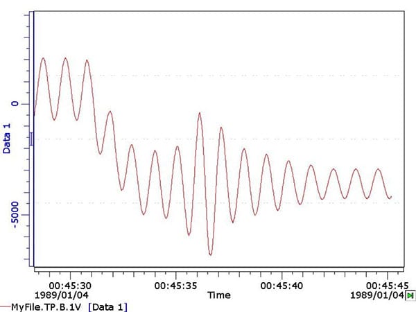
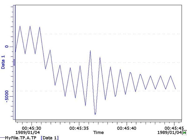
Turning Point Analysis is a method of data compression for arbitrary waveforms. The incoming waveform is sampled at speed and analyzed in real time to identify the turning points (Maxima and Minima) of the waveform, and the value and time of the turning point are also logged to memory for later recovery. The Applications Specialists at CAS DataLoggers have put together this tutorial to examine this subject in detail, including a simple method of noise rejection (dead banding) for dataTaker DT800 and DT500 data loggers.

Applications:

Turning Point Analysis can be used in a large number of applications where a waveform needs to

be monitored. Typical examples include but are not limited to:

• Cyclic fatigue monitoring of structures

• Wave height monitoring of coastal structures / shore erosion

• Tank level monitoring

• Air condition monitoring

• Pressure fluctuations in pipes

• Temperature controller monitoring

Algorithm:

The incoming waveform is sampled and the current data point (n) is compared with the

previous data point (n-1). If the difference between the two samples is positive, then the

signal is rising (a=1), and if negative, then the signal is falling (a=-1).

By comparing the difference of a-1 to a when the signal is rising or falling, a-1 – a = 0.

At the next reading after a maxima turning point, the difference of a-1 – a = 2 and for a minima a-1

– 2 = -2, thus not only giving a clear indication of n-1 being a turning point but also indicating if a

maxima or minima. This technique can also be applied to drawing an envelope around a

waveform.

If n > n-1 then a = 1 (Indicates a rising signal)

If n < n-1 then a = -1 (Indicates a falling signal)

If (a-1)-a < 0 > then n-1 is a valid turning point

In the dataTaker data logger code, this is represented by the command lines:

1CV(DF,=5CV,W)

6CV(DF,=6CV,W)=-1*(5CV<0)+(5CV>0)

The amount of data compression is the ratio of the twice the signal frequency to the sample rate.

I.e. for a 2 Hz signal and 200 Hz sample rate, the compression ratio is 200 / (2*2) = 50:1. This

has a great impact on storage capacity, data efficiency and maximum sampling duration.

Fig 1. Incoming waveform (200Hz, approx. 3400 sample points)

Fig 2. Turning point data extracted in real time (approx. 50 data points)

 

Noise Rejection:

The turning point algorithm is very sensitive and is quite capable of extracting white noise on a

system as actual turning points. This is particularly noticeable when there is a very low frequency

or static signal.

 

To reduce the extraction of noise as turning points, a dead band is applied around the last valid

turning point. If a turning point is detected that has a value inside the range of the last valid

turning point +/- the noise rejection level, then that point is rejected. If the value is outside the

range, then the data point is considered to be valid and is recorded.

While this noise rejection method is simple and effective in most cases, it does

occasionally pick up interim points as turning points. These interim points can be easily identified

and removed in post-processing. Other noise rejection routines will be evaluated and may be

included at a later stage.

DT800 Code:

BEGIN"TP"

'---------------------------------------------------------------------------

' Turning Point Analysis Routine for DT800'

' This code logs the turning points of any waveform.

' The time of turning is recorded logged in 4CV.

'

' Notes: 4CV holds the time since midnight in seconds,

' this limits the time accuracy to 2 decimal places.

'

' Known Issues:

' The noise reduction is primitive and in some instances

' will record false turning points.

' These only happens on occasion and these points can

' be removed by post processing.'

'---------------------------------------------------------------------------'

7CV(W)=10 '7CV hold the dead band for noise rejection

'Any turning points less that the current turning point +/- 7CV will be rejected.

8..9CV(W)=0 'Minimum noise level and Maximum noise level respectively.

10CV(W)=0 'Holds last turning point. Used for noise rejection.

'

' Schedule A is where the turning points are actually logged.

' Note: The X schedule must be before the fast schedule.

'

RAX LOGONA

2CV("TP ~mV",FF7)

4CV("Time ~Sec",FF7)

'

' Schedule B detects the turning point

'

RB,FAST

2CV(W)=1CV 'Shift register for reading

4CV(W)=3CV 'Shift register for time

1V(=1CV,GL20V,W) 'Read Current value (Note: Gain lock to suit)

T(=3CV,W) 'Read current time

1CV(DF,=5CV,W) 'Read difference between readings

 

'This Boolean in the next bit of code returns 1 if the current reading is greater than

'the last (Rising ‘signal) and returns -1 if the current reading is less than the last

'(Falling signal)

'By taking the difference (DF) 6CV holds 2 for a maxima turning point or -2 for a minima

'turning point.

6CV(DF,=6CV,W)=-1*(5CV<0)+(5CV>0)

'Calculate Lower noise tolerance.

8CV(W)=10CV-7CV

'Calculate Upper noise tolerance.

9CV(W)=10CV+7CV

'Then check for turning point and noise then save turning point if valid.

IF(6CV<>-0.5,0.5)AND 'If a turning point AND

IF(1CV<>8CV,9CV){[10CV=2CV XA]} 'If the current signal is outside the noise dead 'band THEN

Record new turning point and Log 'turning point data

END

TN-0015-A0 Page 5 of 6 19 February 2004

 

DT500 Code:

BEGIN

'---------------------------------------------------------------------------

' Turning Point Analysis Routine for DT500'

' This code logs the turning points of any waveform.

' The time of turning is recorded logged in 4CV.

' Notes: 4CV holds the time since midnight in seconds,

' this limits the time accuracy to 2 decimal places.

' Known Issues:

' The noise reduction is primitive and in some instances

' will record false turning points.

' These only happens on occasion and these points can

' be removed by post processing.

'---------------------------------------------------------------------------'

7CV(W)=10 '7CV hold the dead band for noise rejection

'Any turning points less that the current turning point +/- 7CV will be rejected.

8..9CV(W)=0 'Minimum noise level and Maximum noise level respectively.

10CV(W)=0 'Holds last turning point. Used for noise rejection.

'

' Schedule A detects the turning point

'

RA

2CV(W)=1CV 'Shift register for reading

4CV(W)=3CV 'Shift register for time

1V(=1CV,GL20V,W) 'Read Current value (Note: Gain lock to suit)

T(=3CV,W) 'Read current time

1CV(DF,=5CV,W) 'Read difference between readings

'This Boolean in the next bit of code returns 1 if the current reading is greater than the last

'(Rising signal) and returns -1 if the current reading is less than the last (Falling signal)

'By taking the difference (DF) 6CV holds 2 for a maxima turning point or -2 for a minima turning

'point.

6CV(DF,=6CV,W)=-1*(5CV<0)+(5CV>0)

'Calculate Lower noise tolerance.

8CV(W)=10CV-7CV

'Calculate Upper noise tolerance.

9CV(W)=10CV+7CV

‘Record turning point data

RX LOGONX

2CV("TP",FF5)

4CV("Time”,FF5)

RZ

'Then check for turning point and noise then save turning point if valid.

ALARM1(6CV<>-0.5,0.5)AND 'If a turning point AND

ALARM2(1CV<>8CV,9CV)”[10CV=2CV X]” 'If the current signal is outside the noise dead

'band THEN Record new turning point and Log

'turning point data

END